On the Seasonality of Hoppy Beers

Hops are what give beer a bitter, tangy, citrusy, earthy, fruity, floral, herbal, woody, piney, and/or a spicy aromas and flavors. Originally they were used as a preservative because of their natural antimicrobial powers, now they are a defining characteristic of beer. Now with the craft beer movement in full swing they are gaining lots of attention. Hoppy beers like IPAs and pale ales seem to be everyone’s favorites. These days, it seems every brewery is judged on its version of an IPA or pale ale. Everyone is falling behind the view that the hoppier a beer is, the better it must be. I’ve always disagreed with this and come to the realization that I only like a few hoppy beers, and I have to be in the mood for them. This leads me to ask the question, are there more people out there like me? Are hops craved seasonally?

To answer this question, I built an R web scraper to download all the top 100 beers and reviews/ratings/dates for each of those beers (code for that scraper will be posted on GitHub soon). Here is the first six rows of a data set with nearly 90,000 entries:


> head(data)
name date rating state
1 90 Minute IPA 2007-04-09 4.33 Illinois
2 90 Minute IPA 2007-04-07 4.80 California
3 90 Minute IPA 2007-04-02 4.85 Pennsylvania
4 90 Minute IPA 2005-07-03 4.47 Oregon
5 Adam From The Wood 2005-09-12 4.53 Ontario (Canada)
6 AleSmith IPA 2013-09-30 4.20 Wisconsin
review
1 redoing this as my review was unceremoniously...
2 Received in a trade from geexploitation. An excellent...
3 This was really an exceptional beer from start to finish...
4 This IPA pours a beautiful golden color, it leaves...
5 Poured with a medium amount of heat behind it the...
6 The liquid portion is a hazy marmalade orange color...
style abv brewery
1 American Double / Imperial IPA 9.00 Dogfish Head Brewery
2 American Double / Imperial IPA 9.00 Dogfish Head Brewery
3 American Double / Imperial IPA 9.00 Dogfish Head Brewery
4 American Double / Imperial IPA 9.00 Dogfish Head Brewery
5 Old Ale 12.00 Hair of the Dog Brewing Company / Brewery and Tasting Room
6 American IPA 7.25 AleSmith Brewing Company
link
1 http://beeradvocate.com/beer/profile/10099/2093/
2 http://beeradvocate.com/beer/profile/10099/2093/
3 http://beeradvocate.com/beer/profile/10099/2093/
4 http://beeradvocate.com/beer/profile/10099/2093/
5 http://beeradvocate.com/beer/profile/173/20767/
6 http://beeradvocate.com/beer/profile/396/3916/


Yup, the first four entries are for the world famous Dogfish Head 90 minute IPA, a classic representation of this style. What styles are there and what are we including in ‘Hoppy Beers’? The styles I chose are “American Double”, “Imperial IPA”, “American IPA”, and “American Pale Ale”. There are many styles that are hoppy, and you might ask, “What about an English pale ale or an Extra Special Bitter?”, and the reason they weren’t included is that those styles didn’t appear in the top 100 at the time the data was retrieved.

Looking at the exact point plot of ratings over time is meaningless, so let’s look at a smoothed representation of these beers.

AvgRatingOverTime

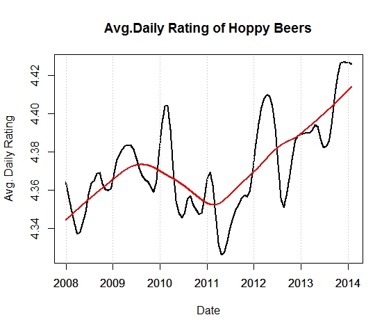
Definitely a trend upwards. This could be the hoppy craft beer culture at work here. What about seasonality? I added an over-smoothed line (in red) to the chart to see the yearly trend. To look at the seasonality within years, let’s subtract the two lines and remove the yearly trend.

AvgRatingDifference

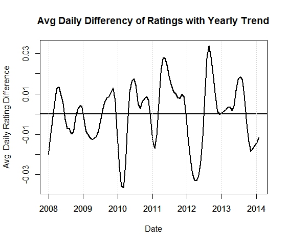
Hmmmm, maybe a possible dip every year in the late winter/spring and a peak in the fall? Interesting. Let’s verify seasonality by finding the peak of the Fourier spectrum of this signal. This will tell us the dominant frequencies in the above time series, which turns out to be around f=0.003006012 days. To find the period of this frequency we invert it to get:

T = 332.67 days.

ALMOST ONE YEAR.

I bet with more data, and controlling for quantity, we could narrow this down to exactly one year. In the future I’m going to do some resampling to figure out the error in the period and hopefully 365.25 will fall within the error bounds. For now, I think I’m going to have a beer.

Cheers.

R code for analysis:


library(TSA) # Time series analysis package
##----Plot Ratings of Hoppy Beers----
hoppy_beerstyles = c("American Double / Imperial IPA","American IPA","American Pale Ale (APA)")
date.seq = seq(from=as.Date("2008-01-01"),to=range(data$date)[2],by=1)
hoppy_ratings_avg = sapply(date.seq,function(x){
mean(data$rating[data$style%in%hoppy_beerstyles & data$date==x],na.rm=TRUE)
})
date.seq = date.seq[!is.na(hoppy_ratings_avg)]
hoppy_ratings_avg = hoppy_ratings_avg[!is.na(hoppy_ratings_avg)]
hoppy_ratings_smooth = lowess(date.seq,hoppy_ratings_avg,f=0.08)$y
hoppy_over_smooth = lowess(date.seq,hoppy_ratings_avg,f=0.4)$y
grid_lines=seq(as.Date("2008-01-01"),as.Date("2014-01-01"), by="+6 month")
plot(date.seq,hoppy_ratings_smooth,main="Avg.Daily Rating of Hoppy Beers",type="l",
xlab="Date",ylab="Avg. Daily Rating",lwd=2)
abline(v=axis.Date(1, x=grid_lines),col = "lightgray", lty = "dotted", lwd = par("lwd"))
lines(date.seq,hoppy_over_smooth,col="red",lwd=2)
##----remove hoppy trend/find periodicity-----
hoppy_no_trend = hoppy_over_smooth - hoppy_ratings_smooth
plot(date.seq,hoppy_no_trend,main="Avg Daily Differency of Ratings with Yearly Trend",type="l",
xlab="Date",ylab="Avg. Daily Rating Difference",lwd=2)
abline(h=0,lwd=2)
abline(v=axis.Date(1, x=grid_lines),col = "lightgray", lty = "dotted", lwd = par("lwd"))
# periodogram(hoppy_no_trend)
hoppy_spec = spectrum(hoppy_no_trend, method = "ar")
hoppy_spec_max = hoppy_spec$freq[which.max(hoppy_spec$spec)]

Posted in analysis, data, R, Webscraping | Tagged , , , | 1 Comment

A Small Trick for Big Data in R

The other day I was writing a prediction script in R for a very large data set. I was data prepping and needed to create a logical vector from a numeric vector. I didn't want to spend the time loading everything into our R-server if I didn't have to deal with that inconvenience. I found a very neat memory saving trick that is quite faster than the normal code.

Let's say you want to create a logical vector from a numeric vector. The logical will be 0 if the numeric is zero and 1 if the numeric is not zero. The obvious way would be to do an if-then statement.


> test = sample(0:10,1000000,replace=T)
> system.time(ifelse(test>0,0,1))
user system elapsed
1.31 0.00 1.31

This may not seem bad, but for my case, I had much more data to deal with, and the regular ifelse statement resulted in a memory overflow. After trying all the normal memory tricks (clearing the workspace, garbage collecting, etc...) with no success, I thought of a better plan.


> system.time(ceiling(pmax(0,pmin(test,1))))
user system elapsed
0.19 0.01 0.20

Nice. This is a nested vectorized min in a vectorized max function, wrapped in a ceiling function. This will work for all non-negative values. But we can go quicker. Of course there are many ways to skin the proverbial cat in R, and the fastest I've found so far is:


> system.time(test[test!=0]<-1) user system elapsed 0.13 0.02 0.14

This works with all numeric values, is quicker, and uses the same storage space. The only downside of this type of command is that it overwrites the numeric field. To work around that just duplicate the column or vector of interest beforehand.

Posted in analysis, data, R | Tagged , , | Leave a comment

Webscraping in R: Part 1

It's hard to believe, but webscraping in R can be done really easily. With no fancy packages either. I recently ran into the need to scrape weather information from the web. After writing the program, I realized this specific task was quite easy compared to other webscrapes. So I decided to make it a post here and show the steps. Soon, I'll write a more complicated webscrape, but for now this will get us started.

To get simple weather data, Weather Underground provides an almanac link which has an option to view in CSV form.

Let's say that I'm interested in a specific date for the weather in Las Vegas. The first step is to find the web address. After some simple searching, the csv file is located at:

"http://www.wunderground.com/history/airport/KLAS/2014/3/09/DailyHistory.html?format=1"

It's important to look and understand the link provided. If need be, explore more CSV links from different dates/cities. It turns out that the 'KLAS' part of the link represents the Las Vegas location. It's pretty obvious the '...2014/03/09...' part of the link represents the year/month/day of the date queried.

Using this information, we can write a simple R script to retrieve this information and save it in a data frame.


##----Set working directory----
setwd("C:/Users/Nick/FromData/Rcode")
##----Set Location Code----
loc_code = "KLAS"
##----Set Retrieval Date----
retrieval_date = as.Date("2014-03-09") # Could also be today: 'Sys.Date()'

Now we need to piece together the site address. To do this we'll use the 'paste' R command.


##----Set Site Address----
# Site = "http://www.wunderground.com/history/airport/KLAS/2014/3/10/DailyHistory.html?format=1"
site_prefix = "http://www.wunderground.com/history/airport/"
site_suffix = "/DailyHistory.html?format=1"
weather_link = paste(site_prefix,loc_code,"/",gsub("-","/",retrieval_date),site_suffix,sep="")

Let's go out and get that data! We'll use the R command 'readLines' to take the information from the web.


##----Retrieve Web Info----
weather_info = readLines(weather_link)[-1]

The '[-1]' is included because R sometimes sticks in a blank first line when using 'readLines' on a website. Now we have 24 rows of one string. Each string contains all the information we need (14 metrics) separated by a comma. Let's parse it up and extract the headers.


weather_info = strsplit(weather_info,",")
headers = weather_info[[1]]
weather_info = weather_info[-1]

Now we have a 24 element list that contains the vectors we want. Let's transform it into a data frame and label the columns with the headers we saved.


weather_info = do.call(rbind.data.frame,weather_info)
names(weather_info)= headers

We are essentially done, except the data frame is comprised of all factors. Not ideal. What we really need is to look through it, determine which columns we want to be numeric, and which ones we want to be strings and convert the corresponding columns. We do this by initially converting everything to a string (using lapply and as.character functions). Then we'll specify which ones are numeric, convert them and then do some date/time clean up.


##----Convert Data Frame Columns----
weather_info <- data.frame(lapply(weather_info, as.character), stringsAsFactors=FALSE) numeric_cols = c(2,3,4,5,6,8,9,10,13) weather_info[numeric_cols] = lapply(weather_info[numeric_cols],as.numeric) weather_info[is.na(weather_info)]=0 colnames(weather_info)[14]="Date" weather_info$Date = as.Date(substr(weather_info$Date,1,10))

Done. This R script can be found in a complete file under my Github account.

For completeness, and because I like graphs, let's look at what the hourly temperature was like on March 9th, 2014.


plot(weather_info$TemperatureF,type="l",main="Temperature",ylab="Temp",xlab="Hour")

Temp_LV_March11th

Yes, it seems that the Las Vegas "winter" isn't really a winter at all. Seventy five degrees in early March.

Posted in analysis, data, R, Webscraping | Tagged , , | Leave a comment

Using DPLYR in R: A Quicker, Easier Way to Work with Data

As I promised, I thought I would show an example using DPLYR. I decided to create my own data set, instead of going with a canned data set in R. I did this to preface my next few posts. After this post, I will be switching to webscraping in R and analysis of beer reviews. I know, I'm excited too.

The data I decided to use is a data set that I recently got by webscraping a very popular beer review site that publishes a highly respected top-250 beer list. It's not a terribly large data set, but it will illustrate the usefulness of DPLYR and answer a question I've always had about beer. That question we will answer is: "Does the abv of a beer influence the rating of a beer?"

I will make the beer webscraper available soon on my github, but I want to optimize the code first. But since I got it working, I downloaded a top 250-beer list and all the reviews/dates/ratings for those beers. Let's take a look at the data.


> str(data)
'data.frame': 72971 obs. of 9 variables:
$ name : chr "90 Minute IPA" "90 Minute IPA" "90 Minute IPA" "90 Minute IPA" ...
$ date : Date, format: "2007-04-09" "2007-04-07" "2007-04-02" "2005-07-03" ...
$ rating : num 4.33 4.8 4.85 4.47 4.53 4.2 4.51 4.48 4.34 4 ...
$ state : Factor w/ 165 levels "","0","Alabama",..: 22 12 49 48 47 65 32 43 38 13 ...
$ review : chr "redoing this as my review was unceremoniously deleted (BA tip: never, ever complain at all if your avatar, and free speech righ"| __truncated__ "Received in a trade from geexploitation. An excellent beer in my opinion. When pouring, I thought it looked a little lite and p"| __truncated__ "This was really an exceptional beer from start to finish. I can't say enough about it. Absolutely remarkable drinkability and b"| __truncated__ "This IPA pours a beautiful golden color, it leaves a nice sticky white lace that sticks to the side of the glass. The smell is "| __truncated__ ...
$ style : Factor w/ 37 levels "American Amber / Red Ale",..: 4 4 4 4 30 7 7 7 7 7 ...
$ abv : num 9 9 9 9 12 7.25 7.25 7.25 7.25 7.25 ...
$ brewery: chr "Dogfish Head Brewery" "Dogfish Head Brewery" "Dogfish Head Brewery" "Dogfish Head Brewery" ...
$ link : chr "http://beeradvocate.com/beer/profile/10099/2093/" "http://beeradvocate.com/beer/profile/10099/2093/" "http://beeradvocate.com/beer/profile/10099/2093/" "http://beeradvocate.com/beer/profile/10099/2093/" ...

So we are dealing with about 70,000 observations of ratings/reviews for the top 250 beers. And yes, the first reviews there are for the famous Dogfish Head 90 Minute IPA. Yum. I'm getting thirsty already.

Back to 'dplyr'. dplyr introduces something that should be standard in R: converting data frames to a non-printable data frame. One of my pet peeves is accidentally asking R to print out a LARGE data frame, and eating up memory, CPU, and time. Check out the fix.


> data_dplyr = tbl_df(data)
> data_dplyr
Source: local data frame [72,971 x 9]
name date rating state
1 90 Minute IPA 2007-04-09 4.33 Illinois
2 90 Minute IPA 2007-04-07 4.80 California
3 90 Minute IPA 2007-04-02 4.85 Pennsylvania
4 90 Minute IPA 2005-07-03 4.47 Oregon
5 Adam From The Wood 2005-09-12 4.53 Ontario (Canada)
6 AleSmith IPA 2013-09-30 4.20 Wisconsin
7 AleSmith IPA 2013-09-30 4.51 Massachusetts
8 AleSmith IPA 2013-09-29 4.48 New York
9 AleSmith IPA 2013-09-15 4.34 Netherlands
10 AleSmith IPA 2013-09-15 4.00 Colorado
.. ... ... ... ...
Variables not shown: review (fctr), style (fctr), abv (dbl), brewery (fctr), link (chr)

Nice. No more little nagging care about accidentally printing out data frames. AND you can do all the same operations on the new 'tbl_df' object as the regular data frame object.

I'm going to compare base R with dplyr in ordering data, selecting subsets, and mutating data by comparing system times for each. Let's look at ordering.


> system.time(arrange(data_dplyr,name,date,rating))
user system elapsed
0.10 0.00 0.11
> system.time(data[order(data$name,data$date,data$rating),])
user system elapsed
0.33 0.00 0.32

This is actually quite the speed up. dplyr's arrange function is about THREE TIMES FASTER than the base function order. AND this isn't that large of a data set. Zoinks, Batman! Let's do this with selecting subsets:


> system.time(select(data_dplyr,name,brewery,state))
user system elapsed
0 0 0
> system.time(data[c("name","brewery","state"),])
user system elapsed
0.08 0.00 0.08

Ok, so my system is obviously rounding down on the first time, so we can safely assume that the first time is less than 0.005 seconds. You might not notice much of a time difference here, but increase the size 1000-fold, and the difference between 80 seconds and 5 seconds is huge.

Let's say that I'm interested in the average rating of a beer PER abv. That means that I have to tell R that I want to take the rating value and divide it by the abv value for each row. (I realize there's a quicker pre-processing method, but for now, let's stick to this example for illustrative purposes). Comparing the times:


> system.time(mutate(data_dplyr,rating_per_abv = rating/abv))
user system elapsed
0 0 0
> system.time(data$rating/data$abv)
user system elapsed
0.01 0 0.01

Ok, so R-base is very close here, I can guess that we are about halving the time.

Let's use some more dplyr functions to see how the ratings of each beer relates to the ABV. The first thing we are going to do is use the group_by function to group our data frame by beer name. Then we will create a summarized data frame of interest that contains the number of reviews, average rating, and the abv.


> abv_rating_data = group_by(data_dplyr, name)
> rating_info = summarise(abv_rating_data,
count = n(),
rating_sum = mean(rating,na.rm=TRUE),
abv_sum = mean(abv,na.rm=TRUE))

Now let's load ggplot2 and make a nice plot with a smooth lowess line to illustrate a relationship.


> library(ggplot2)
> rating_info = filter(rating_info,abv_sum<20) > ggplot(rating_info, aes(abv_sum,rating_sum)) + geom_point(aes(size=count), aplha = 0.7) + geom_smooth() + scale_size_area()

This will create the nice looking graph:

rating_vs_abv

Yay! That was easy enough. What does this graph say? Maybe we can infer that from 4% abv to 12% abv, there's evidence for a very slight overall upward trend, but mostly no observable trend. (Notice that the sample size for beers > 12% is VERY small).

Cheers!

Posted in analysis, data, R | Tagged , , , | Leave a comment

Fast Data Frame Modification in R

One of the frequent data structures I use in R is a data frame. Data frames are similar to matrices except they allow different types of variables in each column. I always rejoice when I can reduce the analysis at hand to a matrix of numbers. R is inherently faster at dealing with matrices than data frames. When I get data that is millions of rows long and over a hundred columns big, R still works, but slows down significantly. Lately, I spend most of my time figuring out the fastest way to transform data and perform calculations on big data frames.

Here is a great solution from the folks at R-studio. I had to post this to get the word out.

Introducing dplyr

'dplyr' is a package that extends the plyr package to data frames and increases the speed tremendously. I plan to post examples using this new package soon.

Posted in analysis, data, R | Tagged , , , , | Leave a comment

Short Circuiting Logical Statements in R

Short circuiting logical statements are the way ‘lazy’ programming languages evaluate logical statements.  To identify whether or not the programming language you are using is lazy or eager, reference the chart on the wiki page: http://en.wikipedia.org/wiki/Short-circuit_evaluation

The lazy (and quicker) way of evaluating logical statements is if any of the logicals joined with an ‘AND’ are false, the whole statement is false.  Conversely, if any of the logicals are joined with an ‘OR’ and any are true, the whole statement is true.  Eager programs will evaluate the whole statement before moving on, and lazy programs will move on as soon as one of those conditions are hit.

Python is, by default, a lazy program and has no options for eager evaluation (although you could explicitly program out eagerness in python).  R has both.  Yup, we should have seen this coming being as R has FIVE different assignment operators (http://stat.ethz.ch/R-manual/R-patched/library/base/html/assignOps.html). The ways to write them are ‘&’ (AND) and ‘|’ (OR) for eager evaluation methods. ‘&&’ (AND) and ‘||’ (OR) for lazy evaluators.

Mandatory python announcement: The logical operators are simply ‘and’ and ‘or’ (written exactly like that) and are by default lazy.  In my opinion, this is a big advantage that python has over R: Simplicity.

Anyways, back to R.  Let’s implement this to show that these operators do indeed work how they should. Remember that testing for equality between a NULL value and a numeric value will return an error in R.

Eager evaluation:


> if(5!=5 & NULL==5){print("This is true!")}else{print("This is false!")}
Error in if (5 != 5 & NULL == 5) { : argument is of length zero

Lazy evaluation:


> if(5!=5 && NULL==5){print("This is true!")}else{print("This is false!")}
[1] "This is false!"

This should raise an eyebrow for a few reasons. Besides being really cool, it is also dangerous. If I’m testing a program with lazy evaluation, it will not output an error if it ends up comparing NULL values to numeric values. Hence good procedure is to test programs with eager evaluation and then switch to lazy evaluation after testing.

Now, I promised an application to big data. When working on big data and we need to go though and test criteria on a very large data set, it’s fair to say that lazy evaluation will be quicker than eager evaluation. Let’s see by how much.


> test.mat = matrix(rnorm(1000000),nrow=1000)
> system.time(apply(test.mat,1,function(r) sapply(r,function(c) if(c>0.99 & c<0.999){c}else{0}))) user system elapsed 5.27 0.00 5.38 > system.time(apply(test.mat,1,function(r) sapply(r,function(c) if(c>0.99 && c<0.999){c}else{0}))) user system elapsed 4.15 0.00 4.24

On one million elements, testing each one by one for two conditions we saved a whole second! Now let’s up the ante.


> system.time(apply(test.mat,1,function(r) sapply(r,function(c) if(c>0.99 & abs(c**2+3*c-2)<0.999 & sin(tan(abs(pi*c)))>0.5){c}else{0})))
user system elapsed
11.43 0.00 11.50
> system.time(apply(test.mat,1,function(r) sapply(r,function(c) if(c>0.99 && abs(c**2+3*c-2)<0.999 && sin(tan(abs(pi*c)))>0.5){c}else{0})))
user system elapsed
4.90 0.00 4.98

We saved over half the time! The above example should help point out that the easier to evaluate logical statements should come first in evaluation to speed up the calculation.
As a side note, please do NOT use short circuiting logical statements when selecting a subset of data. See the following example as to why.


> data = data.frame("a"=c(1,3,5),"b"=c(2,4,6))
> data
a b
1 1 2
2 3 4
3 5 6
> data.subset = data[data$a==3 && data$b==4,]
> print(data.subset)
[1] a b
<0 rows> (or 0-length row.names)
> data.subset = data[data$a==3 & data$b==4,]
> print(data.subset)
a b
2 3 4

You can see that using the short circuiting logical statements reduce our data set down to nothing. Hence, we need to use eager logical statements when sub-setting data.

To summarize, we use lazy evaluation to make programs run quicker with larger data sets and we use eager evaluation to test programs and for sub-setting data.


Posted in analysis, data, R | Tagged , | Leave a comment

Big Data Introduction

Happy Holidays!

For the next few posts, I will be talking about using some tools/tricks on big data. I think that the term 'big data' gets thrown around a bit much these days. The more common definition of big data is any data where it's size presents problems when analyzing it. At work, I have access to a server and Hadoop so the sizes that give me problems are a lot bigger than at home with my workstation. There are a few ways to deal with big data:

  1. Subset the data and work with only the data you need.  Surprisingly, many people don't realize the usefulness of this.  Get rid of those extra columns!  Get rid of missing data!  Get rid of outliers!  Many times, reducing data sets properly solves the big-data problem and not much information is lost.
  2. Get bigger hardware.  My primary tool, R, is a memory based program.  This means all of it's work is done in memory.  That makes it fast but limited.  Not quite 'excel' limited, but limited none-the-less.  Currently, I usually only work with up to about 4-6GB of data in memory.  Since I do have server access at work, I can deal with up to 60-90GB of data.  Still, the more data, the slower any program will run.  If the analysis is quite complicated, we should move on to other options.
  3. Use software that can handle big data.  This means Hadoop (Hive, Pig, Impala), Python, C++/#, etc... . Some also argue that the ff/bigmatrix packages in R work well, and they do to a point.  After trying to get more complicated analyses to work in ff/bigmatrix, I just feel as if I'm tricking R and patchworking/duct taping things together.
  4. Be smart.  If you can write programs that are efficient and fast, you will thank yourself later.  Stay away from loops!  Learn your apply functions.  This type of smart-programming can get you quite far.

Next, I will be posting on being smart in R with short-circuiting logical statements.  They are way cool.

Posted in analysis, data | Tagged , , | Leave a comment

The Simplicity of Python (an example)

Previously, I posted on how to forward fill missing data in columns of data in R and Excel. I just figured out how to do this in Python, and was blown away. Ready?


data = Series(['A','B','C','D','E','F'], index = [0,2,5,7,12,14])
data.reindex(range(14),method='ffill')

Done! It's as simple as telling Python, "Hey I want to reindex the 15 items (0-14) with a forward-fill method". And Python responds, "Done".

Me: "OK, Jump!"

Python: "How high?"

Also, I should mention that "method='bfill'" is... you guessed it... a backwards fill method. Enjoy.

ps- I think that the more I post about Python, the shorter my posts will be. (Thanks to the simplicity of Python).

Posted in analysis, data, Python | Tagged , | Leave a comment

Intro to Survey Analysis

Lately, more people have approached me with questions on how to analyze survey data. There are very interesting problems associated with survey analysis. In dealing with surveys, I have seen mistakes made in creating them. Here are some general rules to follow when making surveys.

  1. For multiple choice answers, make sure that your intended audience always has an option to answer, even if that means incorporating an “other” answer.
  2. If you are performing pre and post survey analysis, do not differ in your categorical questions even the slightest.  E.g. if the pre-survey asks:
    1. What is your income? A)<20K    B) 20-50K    C) >50K

    Then make sure your post survey has the exact same phrasing and answers.  This helps with analyzing the effects before and after an experiment.

  3. Be careful with using too many short-answer or write in answers.  Before you know it all of your analysis will be using text mining to answer questions.  Text mining can be very hard and complicated.
  4. Keep questions short and simple.  The more you confuse your target audience, the more confusing your results will be.
  5. If you are using a rating-scale throughout the survey, be consistent.  Surveys that switch rating scales tend to confuse the audiences.
  6. Low response rates lead to bias.  Try to get a large audience (See # 7).
  7. I always encourage incentives for surveys.  Just be careful that the incentive doesn’t make your audience biased.  E.g. offering an entry for a tablet drawing could draw a younger, more tech-savvy crowd.  If that doesn’t impact your audience, then go for it.

I will not cover things related to determining audience, supervising data collection, obtaining consent, etc.

When it comes to the actual analysis, the first part is data entry.  This is a time consuming, monotonous, and generally torturous activity.  Depending on the size of the audience and response, there are a few options.

  1. Manual labor: If you are an academic researcher, you can probably offer undergraduate credits for data entry.  If not, then you are either on your own, or you can hire someone to help you.
  2. Software conversions:  There exists software to convert paper surveys or electronic documents into data.  They can range from free to expensive, but beware; you get what you pay for.  This method will probably involve lots of data janitoring (Yes, go ahead and add the word janitoring to your word/phone dictionary).
  3. Website Survey Services:
    1. Surveymonkey
    2. Fluidsurveys
    3. Sogosurvey
    4. Wufoo
    5. Surveymoz
    6. Smartsurvey
    7. Surveygizmo
    8. Surveyanalytics

I highly recommend using one of these online services.  They help you create the survey, do data entry, and even do some simple high level analysis for you (summary statistics mostly).

Now we get to move onto data janitoring.  Some data entry methods are probably more prone to errors than other methods.  Software data entry, in which programs try to determine what people have physically written down are the most prone to errors and will require some heavy data cleanup.  Manual entry is probably the easiest as the data should be clean to start with and in a form that is pretty easy to use.  The survey websites will deliver clean data, but some data janitoring might be needed to get the data in a useable form.

In order to do analysis, most surveys will require dealing with silly human errors.  Spelling errors, grammatical errors, abbreviations, and more will make it hard to do analysis.  If you have write-in/short answer questions you have two options to overcome this problem.  The first is overcoming it with a large enough sample size, such that one person writing “This place rox” will not have an impact on the many others who write “This place rocks”.  The second option, given a smaller data set, is to run spell check.  Be careful with this option because spell check can be overactive.  For example, if people write proper nouns starting in lowercase, spell check will want to look for English words to replace them.

Finally we have arrived at the data analysis part.  Give yourself a pat on the back, the hard stuff is over.

Posted in analysis, data | Tagged , , | Leave a comment

The Continuous Breeder's Equation

The Breeder's Equation has always fascinated me. I worked a bit with this equation in graduate school, and now that I'm free to work with whatever interests me at the moment, so I thought I would bring this back up. This equation is as follows:

R=h^{2}S

This equation tells us the phenotypic response (R) in a population generation under some selective force (S) which depends also on the heritability (h) of the trait. A naive example is to consider a trait that is fully heritable (h=1), then the response in a generation is exactly equal to the selected trait. Unfortunately, most traits have heritability that fall somewhere between 0 and 1, this is the hard part to figure out. But all we have to do is wait a generation of intense selection and see the proportion of the population that follows the selection and we have our heritability. This is well-played out with controlled populations that breed discretely (e.g. agriculture products like corn, soybeans, cows...). Like it or not, we have been performing genetic modification of species ever since mankind changed from a hunter/gatherer society to an agriculture based society thousands of years ago. A farmer would always keep the best crops and use them for reseeding next year. Doing this, she imposes a selection force on the population towards a desired characteristic she wants. What about other populations that don't breed/reproduce so discretely? You might even suggest that wild, uncontrolled populations tend to breed discretely as there are many wild animal populations that have a yearly breeding season or two. But let's widen our scope. Most of the life on this planet is single celled organisms. Bacteria, archea, single celled eukaryotes, etc... these populations definitely do NOT breed discretely. If you consider a whole population of bacteria, at any moment in time, there are many cells in various stages of reproduction (assuming a growing population). This equation can NOT be applied to such a population.

In mathematics there are a few ways to convert discrete equations to continuous. But we have to unravel the breeder's equation first. Let's consider it as follows.

(\mu_{o}-\mu)=h^{2}(\mu_{p}-\mu)

Here, the response, R, equals a difference in population means, is the mean phenotypic trait of the offspring generation, is the mean phenotypic trait of the parent generation (that we are selecting for), and the mean of the population as a whole. Again, a quick sanity check (h=1) will give us , a purely heritable trait. Now I want to write the equation to include time. We assume that is the 'generation time' of the population.

(\mu(t+g)-\mu(t))=h^{2}(\mu_{p}-\mu(t))

or

\frac{(\mu(t+g)-\mu(t))}{g}=\frac{h^{2}}{g}(\mu_{p}-\mu(t))

I think you can see how this is going to work. Now we want the limit as and we'll arrive at a continuous derivative.

\frac{d\mu}{dt}=\mu^{'}(t)=\frac{h^{2}}{g}(\mu_{p}-\mu(t))

This non-homogeneous first order differential equation is solvable with the condition that . I'll save you the fun details that you can find in any differential equations book and skip to the answer.

\mu(t)=\mu_{p}\left[ 1+ \left( \frac{\mu_{0}}{\mu_{p}} -1 \right) e^{-\frac{h^{2}}{g}t} \right]

This is a very interesting equation. Let's look at a graph of the situation where the heritability (h) = 0.5, the generation time (g) = 1 unit, the starting phenotypic trait () is 1 and we are selecting for a phenotype of 2 ().

HeritabilityExample

This graph looks exactly as we would expect the population to behave- over time the population approaches the phenotypic value we select. I hope to find some actual data out there soon that approximates this curve. But I'll save that for later, as I don't feel like combing through evolutionary microbiology articles right now.

Posted in Genetics, Microbiology | Tagged , | Leave a comment