Separating Blocks of Numbers in Columns of Data

More and more I'm using the 'apply' functions in R (apply, mapply, sapply, lappy,...). The help functions on these are hard to decipher. Not till I read a post by Neil Saunders, did I really start using them instead of loops.

Lately, I've been creating more nested-apply functions, i.e., an apply function within an apply function. The latest nested apply function I created does something really neat with specific data. What it does is create a list of indices in a sparse matrix down columns of blocks of numbers. Let's look at a simple example.

Let's say here is our raw data:

BlockNum_data

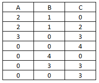
What we are looking to create in R is a list of the block indices of non-zero numbers by column. Here is the function with it's output:


> data = matrix(data=c(2,2,3,0,0,0,0,1,1,0,0,4,3,0,0,2,3,4,0,3,3),
+ nrow=7,ncol=3,dimnames=list(1:7,c("A","B","C")))
> data
A B C
1 2 1 0
2 2 1 2
3 3 0 3
4 0 0 4
5 0 4 0
6 0 3 3
7 0 0 3

The output we seek is a list containing the indices for each non-zero block. For example we want the output for column A to look like:

A[[1]] = 1 2 3 (because the first three positions in column A are non-zero and compromise one block of numbers.

Column B has two blocks, so the output should be:

B[[1]] = 1 2
B[[2]] = 5 6

Here's the nested apply function to create this list (lapply nested inside an apply on the columns).


> list.data = apply(data,2,function(x) lapply(unique(cumsum(c(FALSE, diff(which(x>0))!=1))+1),function(y){
+ which(x>0)[(cumsum(c(FALSE, diff(which(x>0))!=1))+1)==y]
+ }))
> list.data
$A
$A[[1]]
1 2 3
1 2 3
$B
$B[[1]]
1 2
1 2
$B[[2]]
5 6
5 6
$C
$C[[1]]
2 3 4
2 3 4
$C[[2]]
6 7
6 7

Let's break it down step by step. The first thing is to find the non-zero indices. (Let's perform this on the second column, B)


> which(data[,2]>0)
1 2 5 6
1 2 5 6

Remember R reads down columns. Now let's find where non-consecutive differences occur (to separate the blocks).


> diff(which(data[,2]>0))
2 5 6
1 3 1

Notice, wherever there are non-ones is where the break occurs. But because of how the 'diff' function works, we need to add a position in front. Let's also convert them to logicals.


> c(FALSE, diff(which(data[,2]>0))!=1)
2 5 6
FALSE FALSE TRUE FALSE

If we do a cumulative sum of these logicals (remember FALSE = 0, and TRUE = 1) we will have separated the blocks with integers starting at 1.


> cumsum(c(FALSE, diff(which(data[,2]>0))!=1))
2 5 6
0 0 1 1

If we add one and find the unique ones, we get:


> unique(cumsum(c(FALSE, diff(which(data[,2]>0))!=1))+1)
[1] 1 2

Now let's wrap it up in a 'lapply' function to return a list for column B:


> lapply(unique(cumsum(c(FALSE, diff(which(data[,2]>0))!=1))+1),function(y){
+ which(data[,2]>0)[(cumsum(c(FALSE, diff(which(data[,2]>0))!=1))+1)==y]
+ })
[[1]]
1 2
1 2

[[2]]
5 6
5 6

Now we just stick it in an apply function across the columns to find the indices of blocks of non-zero numbers. (Or across rows if you want.)


> apply(data,2,function(x) lapply(unique(cumsum(c(FALSE, diff(which(x>0))!=1))+1),function(y){
+ which(x>0)[(cumsum(c(FALSE, diff(which(x>0))!=1))+1)==y]
+ }))
$A
$A[[1]]
1 2 3
1 2 3
$B
$B[[1]]
1 2
1 2
$B[[2]]
5 6
5 6
$C
$C[[1]]
2 3 4
2 3 4
$C[[2]]
6 7
6 7

Sometimes I get so proud of my nested apply functions... sniff... sniff. One day I hope to write a triple nested apply function. I hope someone finds this useful.

Posted in data, R | Tagged , | Leave a comment

Prime Time Calculation

Number theory has always interested me, specifically irrational numbers and prime numbers.   I was messing around with functions in R and came up with a very neat ‘one line’ function in R that checks if a number is prime.  See below:

IsPrime = function(n){if(n>3){if(any(sapply(seq(2,floor(sqrt(n))),function(x) n%%x)==0)){FALSE}else{TRUE}}else if (n%in%c(2,3)){TRUE} else{FALSE}}

(Bonus Math Karma to anyone that knows why the square root function is in there). To check the function works, here are the first 17 integers checked:

PrimeCheck1

Looks good so far.   This ‘IsPrime’ function checks integers for being prime.  I thought to myself, what are the reaches of this function?  How big of a number can I check with reasonable times/resources?  Let’s create a sequence of very large numbers.

prime.seq.check = 10^(seq(5,14))+1

Note that the vector ‘prime.seq.check’ contains the sequence:

100,001; 1,000,001; 10,000,001; …

And so on, and ends with a 15 digit integer:

100,000,000,000,001 (A hundred billion and one).  What are the times to compute if these are prime?  Let’s use the ‘proc.time’ R-function to loop through and time these.

times = rep(0,length(prime.seq.check))
prime.log = rep(0,length(prime.seq.check))
for (p in 1:length(prime.seq.check)){
tic = proc.time()[3]
prime.log[p] = IsPrime(prime.seq.check[p])
times[p] = proc.time()[3]-tic
print(paste("Done with ",p," out of ",length(prime.seq.check),sep=""))
}

Let’s plot the output:

plot(seq(5,14),times,main="Prime Time Computation", xlab="Number of Digits",
ylab="Seconds in Prime Computation",lwd=2)

ExponentialPrime1

Looks very exponential.  Let’s fit an exponential function using some basic algebra.

x.seq = seq(0,14,by=0.1)
y1 = times[10]
x1 = 14
y2 = times[9]
x2 = 13
b = (log(y1/y2))/(x1-x2)
c = y1/(exp(b*x1))
y.seq = (c)*exp((b)*x.seq)
plot(seq(5,14),times,main="Prime Time Computation", xlab="Number of Digits",
ylab="Seconds in Prime Computation",lwd=2)
grid()
lines(x.seq,y.seq,col="red",lwd=2)
points(seq(5,14),times,lwd=2)

ExponentialPrime2Turns out the function is given by f(x) = (4.082583E-6) * exp(1.220295 * x).  The largest prime to date has 17,425,170 digits.  I used Wolfram Alpha to calculate this, and it would take about 2E9234766 seconds.  MUCH longer than the estimated age of the universe.
 

So, needless to say, this prime number function is not going to help in the search for prime numbers.  But it is cool.


More props to you, pure math.

Posted in analysis, math, R | Tagged , , , | Leave a comment

Quick Data Tip in R and Excel

Last week, a colleague showed me a trick in excel.  And it really bugs me when you can do something in excel that R can not do easily.  So I gave it some thought and came up with a solution.  Here's the problem:

Sometimes we have data with missing values and want to fill them in a specific way.  What if you want to fill them in with the above-nearest non-missing value?  An example of such a data set:

ExcelRRecursionDataYou can imagine that it's easy to do this manually for a small data set, but tedious and horrible for larger data sets.  The instructions for excel is this:

  1. Select data.
  2. Hit F5 (Go To command)
  3. Click on the 'Special...' button.
  4. Select the 'Blanks' option, hit ok.
  5. Now, while every blank is highlighted, type in "=A2", where A2 is your first non-blank value.
  6. Hit 'Ctrl + Enter' at the same time.

Viola!  Done.  This can be done even faster with keyboard shortcuts.

In R, we have to be smart.  But it can be done easily with a recursive function.  See the code below.

##-----Recursive Fill in------
# This script will attempt to do an excel trick with a recursive R function

data = data.frame("label"=c("A",NA,"B",NA,NA,"C",NA,"D",NA,NA,NA,NA,"E",NA,"F"))

non.na.index = function(x,data){if(is.na(data[x])){non.na.index(x-1,data)}else{data[x]}}

new.column = sapply(1:(dim(data)[1]),function(x) non.na.index(x,data$label))

This R code does the following:

  1. Creates the data and the missing rows are designated as "NA". This is standard for R.
  2. non.na.index function takes a column and an index.  If that value is NA, it calls itself for the index above it.
  3. The 'sapply' function is used to apply the function over a whole column.

This runs relatively quick and gives us the same column as the excel trick.  Neat-o.


PS-  If the data comes this way via pivot tables in Excel, remember you can format the pivot tables certain ways to avoid having to do this at all.

Posted in data | Tagged , , , | Leave a comment

Approaching Data Analysis

All data analysis projects start with a problem.  We (hopefully) form a hypothesis before exploring the data, and we go about trying to confirm/disprove hypotheses with statistical procedures.  These statistical procedures could be a simple t-test, a more complicated non-parametric bootstrap, or just producing a visual aid.

Most of the time, working in the industry, people approach me with a solution in mind.  They know what they want to see and need my help confirming their views.  In conversations, I try to back them out of that view point and prepare them for possible alternative outcomes.  This is the point in which I start the data analysis, by trying to understand the problem.  This usually involves defining the problem and variables involved as mathematically/logically as possible.

Mathematics gets it's power from defining things well.  If we truly define our problem well, it will be worlds easier to find a solution.  In fact, historically, major strides in mathematics were due to either a brilliant stroke of genius or a new and more precise way of defining objects and problems.

Once we have covered the problem, we talk about a possible approach.  Most often than not, there are many possible solutions to a problem.  In considering the many methods for solving a problem, remember that the simplest solution can be the best solution.

While talking about arriving at a solution, we should also be talking about the possible sources of data for the problem.  Sometimes the hardest part of a data analysis project is getting the data required.  It is even possible that the lack of data or form of data requires us to change our method for a solution.

Now for the fun part (cue sarcasm), cleaning the data.  As a data analyst, data scientist, or whatever new buzz word is out there (data wrangler?), a majority of your job will be data janitoring, data cleaning, and data formatting.  One harsh aspect of working in the industry is that data is never in the form you want.  This is a skill set that I had to work to develop on my own, as academic data sets never required much cleaning.  This is also one of the most frustrating parts of the process and it also can take a lot of time.  Just sit your butt down and pick your favorite tool/software package and hack away at the data.  As for what to look for, consider the process below.

Data Janitoring

At this time, I recommend doing some sanity and quality checks of the data.  Did you just import a data point for each hour of each day? Check for that.  Check for outliers.  Check for missing data, if there is missing data, is it missing at random?

At this point, the fun begins.  We get to do what we wanted.  Now we can make the data dance, sing, and do headstands at our command.  From this point on, the method of data analysis is very unique to the problem.  But to get started, I always do some sort of initial data exploratory analysis.  This means I produce scatter plots, means, variances, correlations, pivot tables, etc…  This helps me become intimately familiar with the data, which in turn helps me see the quality of the data.

dataAndYou

Let’s recap.

i.            Talk about the problem and ask questions.

ii.            Brainstorm approaches.

iii.            Find data sources, possibly modify approach based on data source.

iv.            Data cleaning and formatting.

v.            Check data for outliers/missing data.

vi.            Exploratory data analysis (become intimate with the data).

vii.            Commence methods to approach solution/test hypothesis.

ppdac

In academia, most of the time we start at step (vi) or (vii) and skip some important stuff.  In the industry, you get to work with people who are not mathematically inclined.  This isn’t a problem unless they are stubborn and refuse to see logic.  Dealing with these people is a whole different problem, and I wish you luck.

Cheers.

Posted in data | Tagged , , , | Leave a comment

Philosophy and Purpose

A little over a year ago, I transferred from working on applied mathematics in academia to working in the industry as a data analyst.  Like any person that leaves the academic bubble, the outside world is very different from expectations.  Working on data analysis in academia and industry both share common goals.  They both aim to solve problems.  But they emphasize different parts of the process.  In my experience, academia focuses more on methods.  They aim to test new methods and delve into unexplored areas of data analysis.  The industry environment focuses more on the solution than the method.  This means that the fancy algorithms and methods we learned in academia are not always the best option.  Having an algorithm that converges to a more accurate solution, but takes more time or more computational power, might not be ideal.

academia-or-industry

I started to run into more and more problems in the industry that have solutions sometimes too obvious to be found.  On the flip side, I have occasionally run into problems that require some intense statistical/mathematical/data analysis to get a handle on.  The idea for this blog is to introduce data analysis for the industry, hopefully helping data analysts (myself included) come to better conclusions.

It is from data that we make conclusions.  We do this every day.  We predict how long our commute home from work will be at a certain hour, pizza restaurants estimate the delivery time of our favorite pizza, weather stations come up with forecasts, etc.  Defining, harnessing, scrutinizing, and improving this prediction power will benefit everyone.

Enough idealism.  The plan is to cover a wide variety of mathematical, statistical, and data analysis topics and show examples and how to implement them.  The software that I am most comfortable with is R, Matlab, Python, and (gasp!) excel.  If you want me to cover a specific topic or have a question about something, feel free to email me or leave a comment.

Posted in Uncategorized | Tagged , | Leave a comment